In this third and final installment discussing TrajectoryLog.NET, we explore the role the TrajectoryLog.NET API plays in analyzing customized QA fields, and how to build creative quality assurance plans to meet your QA needs. The TrajectoryLog.NET API was introduced in a prior blog post as an open-source .NET API that interprets the binary trajectory log files created by Varian linear accelerators during treatment and quality assurance deliveries. A second post highlighted the ability of the TrajectoryLog.NET API to assist in building fluence images for the visualization and comparison between expected and delivered MLC leaf trajectories.
TrueBeam Delivery Logic
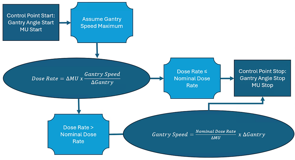
When designing VMAT QA beams for delivery, its useful to review the logic the linear accelerators use to interpret control points. During a VMAT delivery, the control point instructions to the treatment machine include the Monitor Unit value and the gantry angle position. In between the control point position, the Gantry speed is assumed to be the maximum speed with which the linear accelerator can rotate (i.e. 6 degrees/second for the TrueBeam). In this case, the Dose Rate is calculated from the change in Monitor Unit Value multiplied by the maximum gantry speed over the entire gantry trajectory. It could be the case that this dose rate is higher than the nominally selected dose rate for the field. In that case, the dose rate can only hit this ceiling, and the gantry speed will decrease to ensure all the dose can be delivered within a given control point.
Building dynamic QA fields with the Eclipse Scripting API possesses an additional level of complexity to overcome. Within the Eclipse Scripting API, the AddVMATBeam() method will place the gantry angles uniformly between the starting gantry angle and the stopping gantry angle (giving no control over ΔGantry). Instead, all control over the MLC speed, dose rate, and Gantry Speed lies on the total MU delivered for the field and the meterset weight at each control point. To expedite the planning process with ESAPI, a spreadsheet can be used to calculate parameters ahead of time using the information above.
In this hypothetical field, an arc will start at gantry angle 170 and travel to gantry angle 10 in a set of 20 control points. This results in 8 degrees of travel per control point. Assuming a nominal dose rate of 600, we can plan for the total MU of the beam to be 200 MU. Given an evenly distributed 0.05MU per control point, the dose rate will remain a constant 450MU/min and the gantry speed can maintain a maximum 6 degrees/second. Please note the equation in the formula box calculates the expected dose rate for each control point.

To test the behavior of the spreadsheet. Change the Total MU to 1000 MU. The requested dose rate skyrockets to 2250 MU/min! Since the actual dose rate can only be 600MU/min or below, the gantry speed must compensate to allow for the delivery of 5X more dose within each 8 degree span. Please note the equation in the formula box with an if statement logic that calculates the gantry speed from the highlighted values if the requested dose rate is greater than the nominal dose rate.

To cause a difference in the gantry speed, one could simply skew the meterset weights toward one part of the delivered field. For instance, if in the first 10 out of 20 control points, 75% of the MU were delivered instead of 50%, then the second half of the field had the other 25% delivered, then the gantry angle may need to adjust speed in between depending on the total MU delivered for this beam and the nominal dose rate. Also note here the Actual Dose rate calcuation formula is visible.

On a quick note, if the MLC positions were to be in respective positions for each of these gantry speed regions, it would be advisable to allocate some control points with low MU contributions whereby the MLC positions can move from one place to another. For this example, the focus is on testing gantry speed, and the MLC will be a continuously sweeping gap.
Developing the Script
In the example script, a simple stand-alone executable will be created and deployed on an already generated phantom image. Remember as the script is a write-enabled script the assembly attribute tag [assembly: ESAPIScript(IsWriteable = true)] will need to be included above the namespace.

Within the execute method, we will access our patient. This patient is a simple phantom generated in the contouring workspace. Remember to call BeginModifications() on the patient for modifications. Next, add a course and plan on the structure set associated with the patient. When the beam is generated, the meterset weights must be known. A simple for loop can set up the 2-tiered meterset weight values.
// TODO: Add your code here.
//generate course and plan.
Patient patient = app.OpenPatientById("PH_QA_001");
patient.BeginModifications();
Course course = patient.AddCourse();
StructureSet structureSet = patient.StructureSets.First(ss => ss.Image.Id == "PHANTOM3" && ss.Id == "PHANTOM3");

ExternalPlanSetup plan = course.AddExternalPlanSetup(structureSet);

//Build out meterset weights.
List<double> metersetWeights = new List<double>();
metersetWeights.Add(0);

for(int i = 0; i < 20; i++)
{
    if (i < 11)
    {
        metersetWeights.Add(metersetWeights.Last() + 0.075);
    }
    else
    {
        metersetWeights.Add(metersetWeights.Last() + 0.025);
    }
}
A beam can then be added to a programmed machine using the AddVMATBeam() method. The start gantry angle and stop gantry angles are selected from the spreadsheet. Afterwards, the jaw positions can be set to an symmetric 12cm x 36cm field size in the X-Jaw and Y-Jaw, respectively. Finally, the MLC positions are set by looping through the control points of the beam and setting the MLC linearly with the meterset weight that has been defined for that given control point. Finally save the plan for review in Eclipse.
//Add beam
ExternalBeamMachineParameters parameters = new ExternalBeamMachineParameters("TrueBeam", "6X", 600, "ARC", null);
Beam beam = plan.AddVMATBeam(parameters,
    metersetWeights,
    0,
    170,
    10,
    GantryDirection.CounterClockwise,
    0,
    new VVector(0, 0, 0));

//update MLC positions at each control point
var editables = beam.GetEditableParameters();

editables.SetJawPositions(new VRect<double>(-60, -180, 60, 180));
//2cm MLC slit that moves through the field evenly through control points.

foreach(var cp in editables.ControlPoints)
{
    float[,] mlc = new float[2, 60];
    float a_bank = -70f + 120f * (float)cp.MetersetWeight;
    float b_bank = -50f + 120f * (float)cp.MetersetWeight;
    for(int i = 0; i < 60; i++)
    {
        mlc[0,i] = a_bank;
        mlc[1, i] = b_bank;
    }
    cp.LeafPositions = mlc;
}
beam.ApplyParameters(editables);
app.SaveModifications();
Console.WriteLine("Complete!");
Console.ReadLine();
Review the plan in Eclipse.

To finalize the plan, calculate the plan with preset MU. In this example, 300MU is selected to match the excel spreadsheet discussed in the previous section. From the properties of the MLC, it is apparent how similar the results are to the expected results from the excel spreadsheet planning.

Feel free to prepare and deliver the new QA plan!
TrajectoryLog Analysis
In this section, the ToCSV() method of the TrajectoryLog.NET API is explored. Once the plan has been delivered, gather the trajectory log file and generate a new Visual Studio project for the analysis. For a quick analysis, generate a console application in Visual Studio. If it hasn't been done from past use with the TrajectoryLog.NET API, clone the open-source repository as described in the first section of the prior blog post. Add the TrajectoryLog.NET referenced library to the current project. Generate a bit of code to access the trajectory log file an export the file to a CSV.
static void Main(string[] args)
{
		   OpenFileDialog ofd = new OpenFileDialog()
            ofd.Filter = "Trajectory Log File (*.bin)|*.bin";
            TrajectoryAPI.EnableDebug();
            TrajectorySpecifications.TrajectoryLogInfo locallog = null;
            if (ofd.ShowDialog() == true)
            {
                locallog = TrajectoryAPI.LoadLog(ofd.FileName);
            }

            Console.WriteLine("Do you want to write .csv? (y/n)");
            if (Console.ReadLine().Trim().Equals("y", StringComparison.OrdinalIgnoreCase))
            {
                TrajectoryAPI.ToCSV(locallog);
            }

            Console.ReadLine();
}
By copying the MU Actual Row and the Gantry Actual [deg] row and pasting them transposed from another sheet in the CSV file, the gantry speed that was expected and/or the actual gantry speed can be evaluated can be evaluated. The key to evaluating the gantry speed, MLC speed, or dose rate (values that are not included in the trajectory log file directly) is knowing that the trajectory log files are written every 20ms. This allows for the introduction of a time axis in the file.

Comments